In my previous post about setting up the IMX219 stereo module with the Jetson Nano, I claimed that extracting depth maps with OpenCV “shouldn’t be a problem”. Well, this post is about just that. Wide-angle lenses are not exactly optimal for many stereo vision applications as the resolution diminishes quite quickly over greater distances. Stereo matching can also be difficult to perform for points that are close to the cameras, as the corresponding points can look quite different due to the extreme viewing angles of the cameras. Additionally, due to the more severe distortions produced by wide-angle lenses, the cameras are more challenging to calibrate. Due to these reasons it was really interesting to try generating depth maps with the IMX219. Codes are available in my github.

Calibration

Extracting depth from a stereo camera pair requires careful calibration. The intrinsic parameters of both cameras must be solved, as well as the relative transformation between the camera coordinate systems. These camera parameters are utilised to perform the stereo matching in an efficient manner and triangulate the depth. In OpenCV, calibration is convenient to perform with a checkerboard pattern captured from multiple angles with the stereo pair. Here, I used approximately 50 pairs of captured calibration images. The number of samples was a bit extreme, but the wide-angle lenses can be really difficult to calibrate correctly.

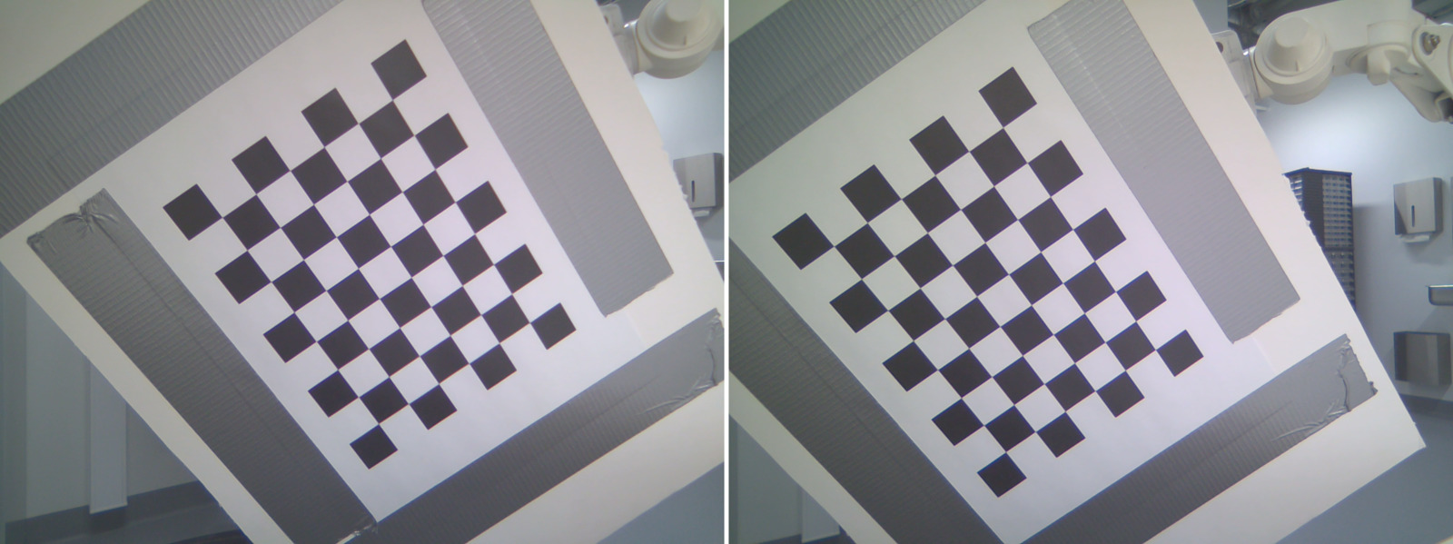
The square size and checkerboard dimensions (as in number of inner corners) are needed as prior knowledge for calibration. OpenCV is used to detect the corners, and the corners’ image coordinates are saved along with the real-world coordinates (generated with the known square size and checkerboard dimensions). Based on this data, I first calibrated both cameras individually. The resulting camera intrinsic parameters were used as fixed inputs for the stereo calibration, in order to limit the number of variables for the numerical optimisation. After finishing the stereo calibration, I had everything I needed to get started with creating depth maps.

Test setup for depth extraction

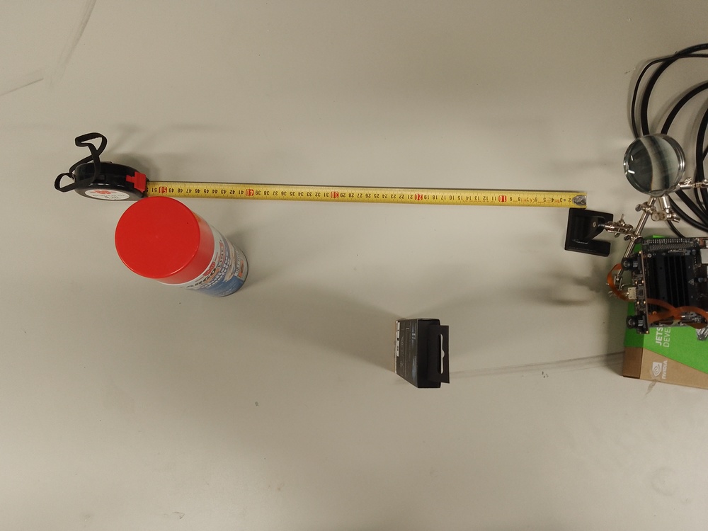
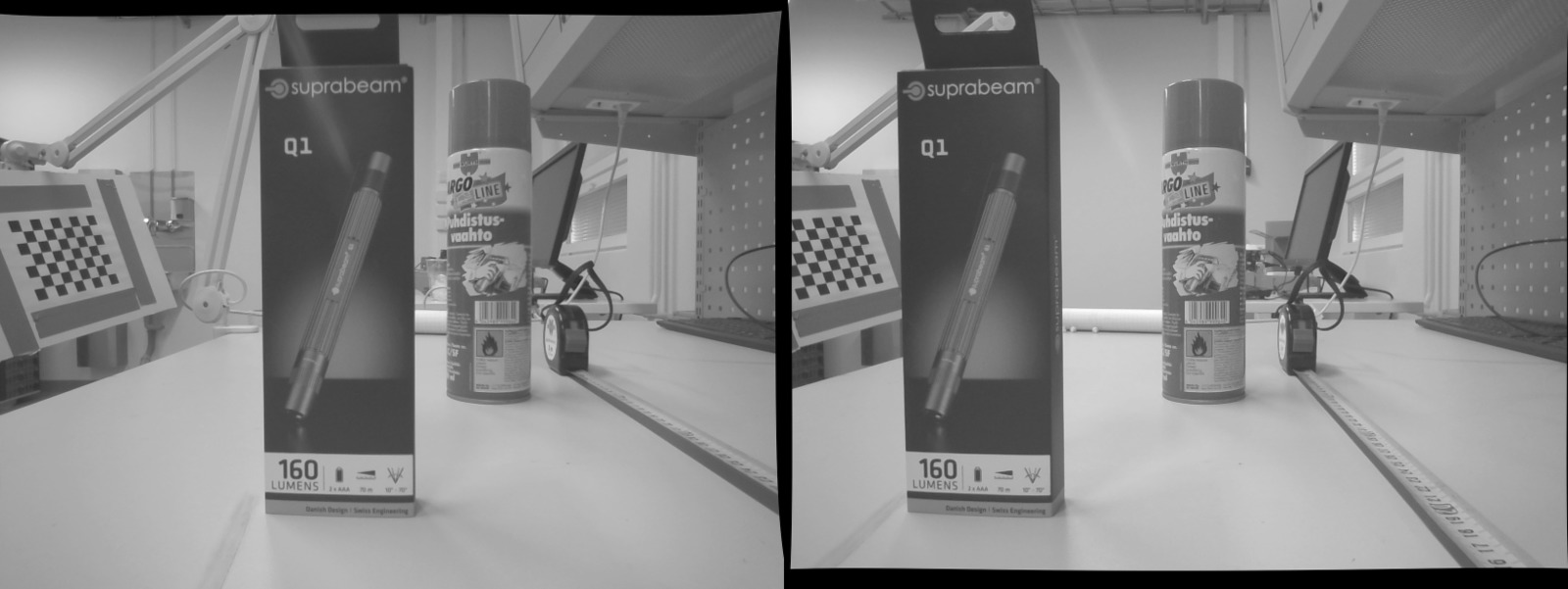
With the stereo camera parameters calibrated, it was time to build a test setup for validating the depth extraction accuracy. I placed a couple of random objects in front of the stereo camera at different distances and a tape measure for reference. Then I captured frames from both cameras for depth extraction.

Stereo matching and depth extraction

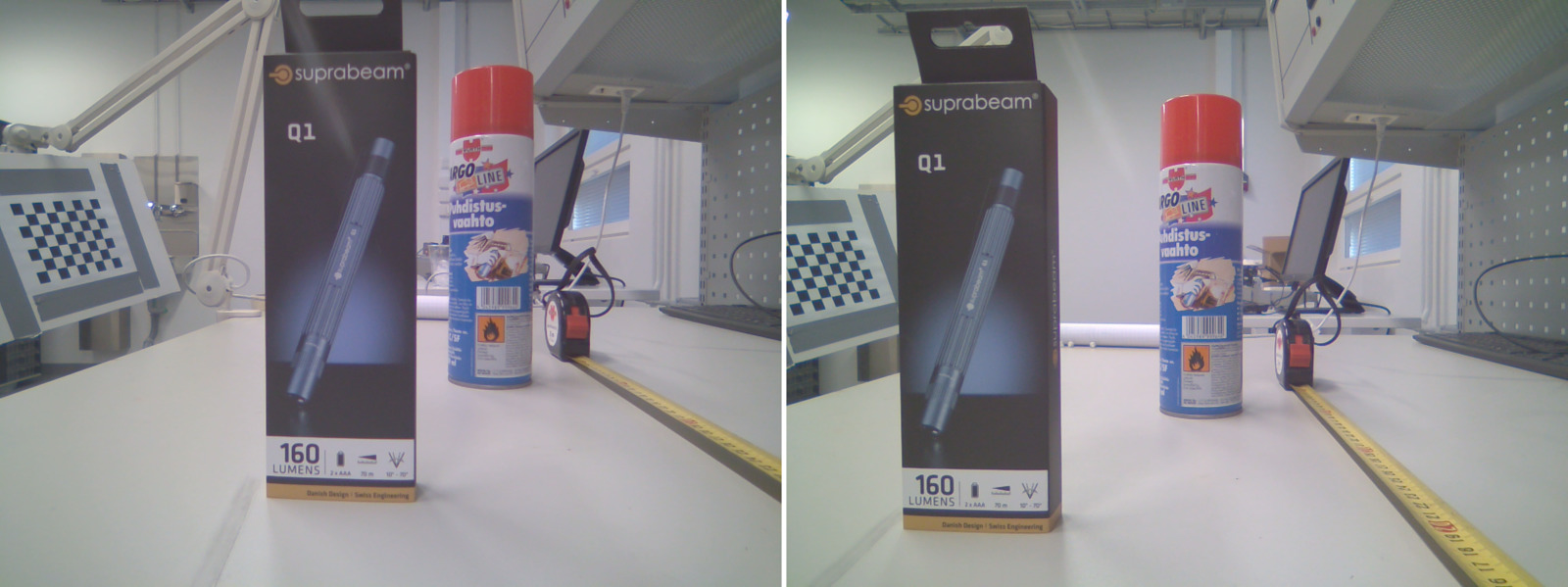
In order to perform stereo matching, the captured images are first rectified, i.e. transformed to a common plane in such a way that they correspond horizontally. This makes the stereo matching task simpler, as the search for matching regions can be carried out on horizontal lines. The rectification is executed with OpenCV, utilising the camera parameters from the calibration.

After performing stereo matching on the rectified camera views and finding the corresponding pixels, the disparities can be computed. More lit (“hotter”) areas indicate areas that are closer, i.e. the disparity is higher. Regions where stereo matching was not successful and correspondence was not found, are illustrated in black. The disparity map is not exactly clean, with loads of areas where the stereo matching has failed. This is likely due to the wide-angle lenses and the difficulty of correctly calibrating them and performing stereo matching with them.

Again using the camera parameters acquired from calibration, the disparity map can be transformed to a 3D point cloud. Below you can see the point cloud generated from the test images. Distant points have been filtered away for a clearer representation. First I visualised the point cloud with Open3D, which handled the large point cloud impressively.

However, I couldn’t find an option in Open3D to visualise a grid that would give me a reference for checking how well the point cloud captured the dimensions of the real world. So, I decided to visualise the point cloud in good old Matplotlib as well. Matplotlib is not exactly the best tool for visualising large amounts of data and I had to trim the point cloud by quite a bit to get visualisation working in a sensible manner.

The Matplotlib visualisation showed that the point cloud captured the real-world dimensions quite accurately. Looking at the picture of the test setup at the beginning of the post, you can read from the tape measure that the cardboard package was at a distance of 20 cm and the spray can was at a distance of 40 cm. The tape measure itself was drawn to a length of around 52 cm. The Matplotlib visualisation shows that the depth of the setup was captured quite well, showing the two objects at their respective distances of 20 cm and 40 cm. The tape measure however appears to be positioned at a distance of approximately 55 cm, so there seems to a bit of error there. This is likely due to the difficulty of wide-angle stereo vision, causing errors that increase over distance. Or it could be due to the fact that I placed the tape measure quite haphazardly, it might have been in a slight angle.