After a friend talked to me very highly of Microsoft Azure and their ML studio, I finally decided to grab their free trial and get acquinted with the cloud platform giant. When it comes to cloud computing, I’ve always built my own server solutions on cloud resources operated by service providers such as Linode. Custom solutions always have the benefit of flexibility, yet implementation can be quite time-consuming. Looking into Azure, I was interested in seeing what type of balance they have found between convenience and versatility. I started by checking out the ML studio, as machine learning is one of my top interests. Via the browser interface I created an ML workspace, and I had plans to create some basic PyTorch model and deploy that in the cloud. However, like a moth to a flame, I was instantly drawn towards the “Automated ML” tab. This type of application has great potential to reduce manual iteration performed by data scientists. Furthermore, a properly automated workflow can more thoroughly search through the applicable algorithms and their hyperparameters.

Automated ML Setup

Kicking off the configuration for an Automated ML job, first I had to select which dataset I was going to use. Browsing the offered open source datasets, I ended up selecting the MNIST dataset of handwritten digits due to my fondness of computer vision. The dataset is not much of a challenge for most classification algorithms, but hey, it’s a classic. Plus the other available datasets didn’t seem that challenging either, it was mostly the basic stuff you’d expect.

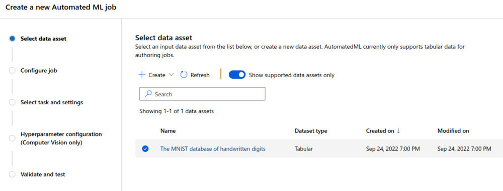
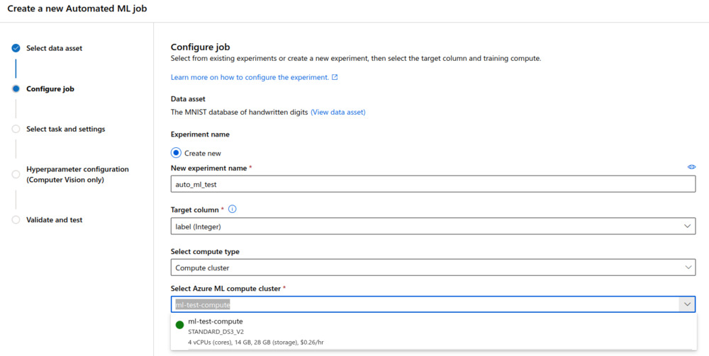
The MNIST data was crunched into a tabular format, with image per row, and the columns representing grayscale pixel values. The last column was reserved for the label, 0-9. Defining the label-column as the ground truth for the classification task, it was then time to select which compute cluster to utilise for doing the heavy lifting. I wanted go for a minimalistic approach, in order to test how computationally efficient they had made the training process. I selected a basic cluster with 4 CPU-cores and a generous 14 GBs of memory.

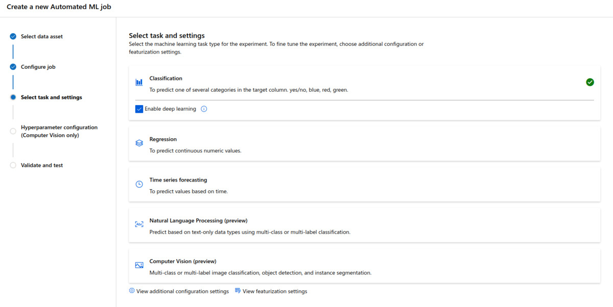
Then it was time to define the type of the machine learning task. Here I was tricked to selecting “Computer Vision” at first, which led to a bunch of error messages. Then I realised the data was in the tabular format, so in reality the task was just generic classification. So, selecting the task as “Classification”, I also checked the “Enable deep learning” box. With the classification task I didn’t get to see what was behind the “Hyperparameter configuration”-page. Considering only tabular data was supported at the time of writing, I’m not really sure how one could configure a computer vision-task.

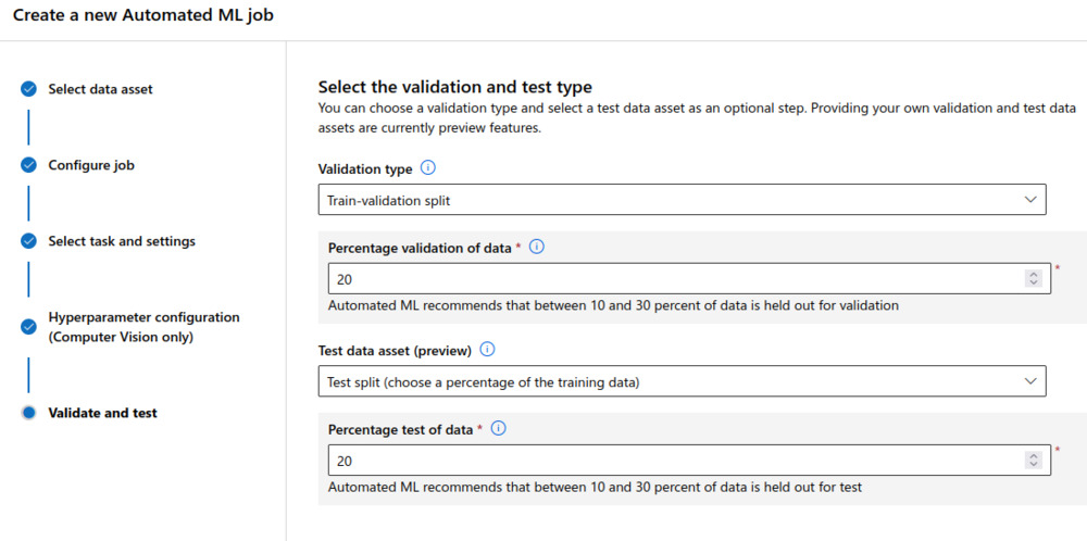
As a final step I split the validation and test sets, sampling both as 20/% portions of the available data. A total of 70 000 images were available in the MNIST dataset. I chose quite large validation and test sets, as I was interested in analysing the performance, rather than trying to train the most universally accurate model.

After this, the job was created and I left it running on the compute cluster. I was expecting that I’d see the result in a day or two, considering the modest resources provided for the job.

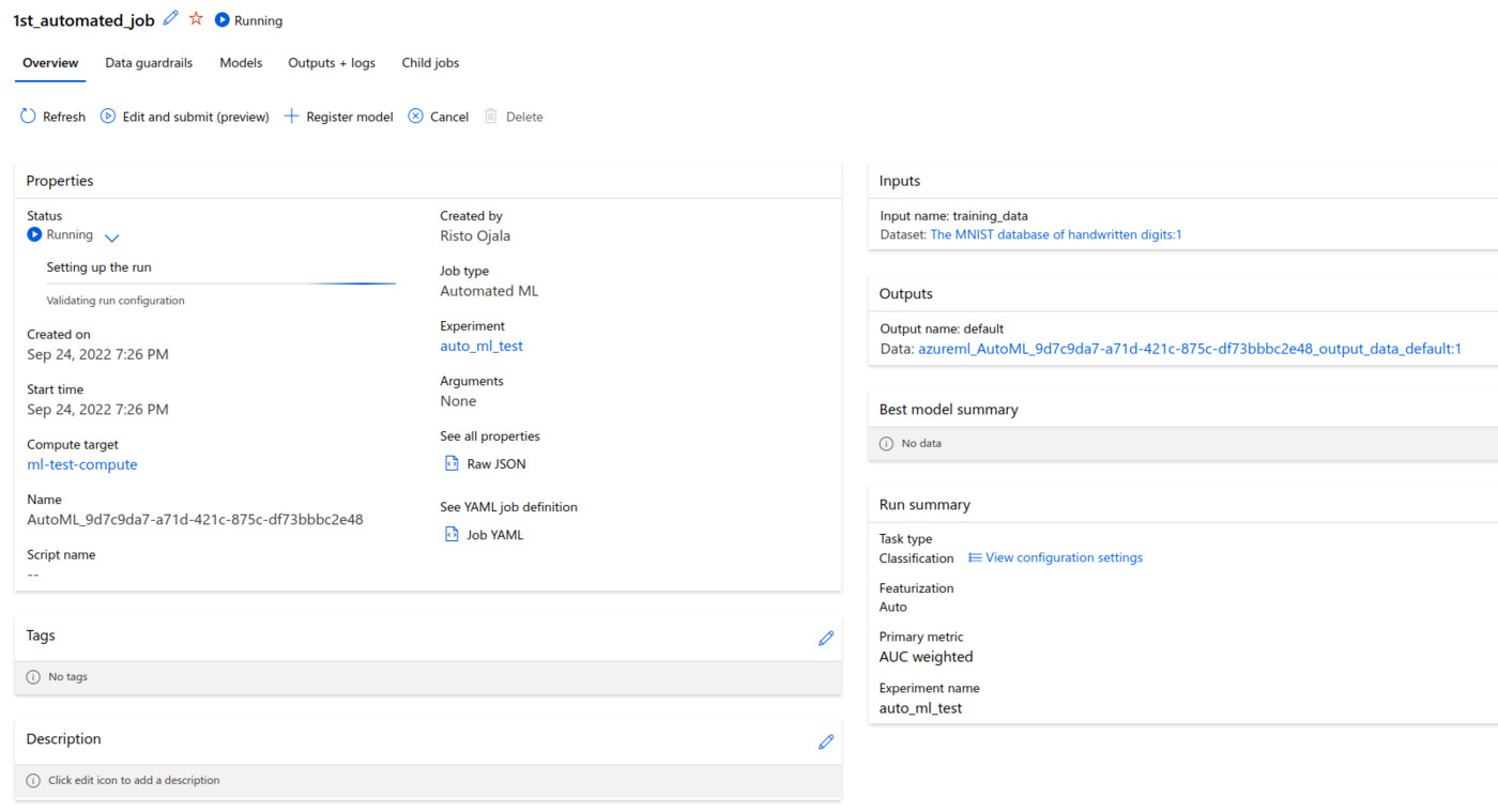
Automated ML Results

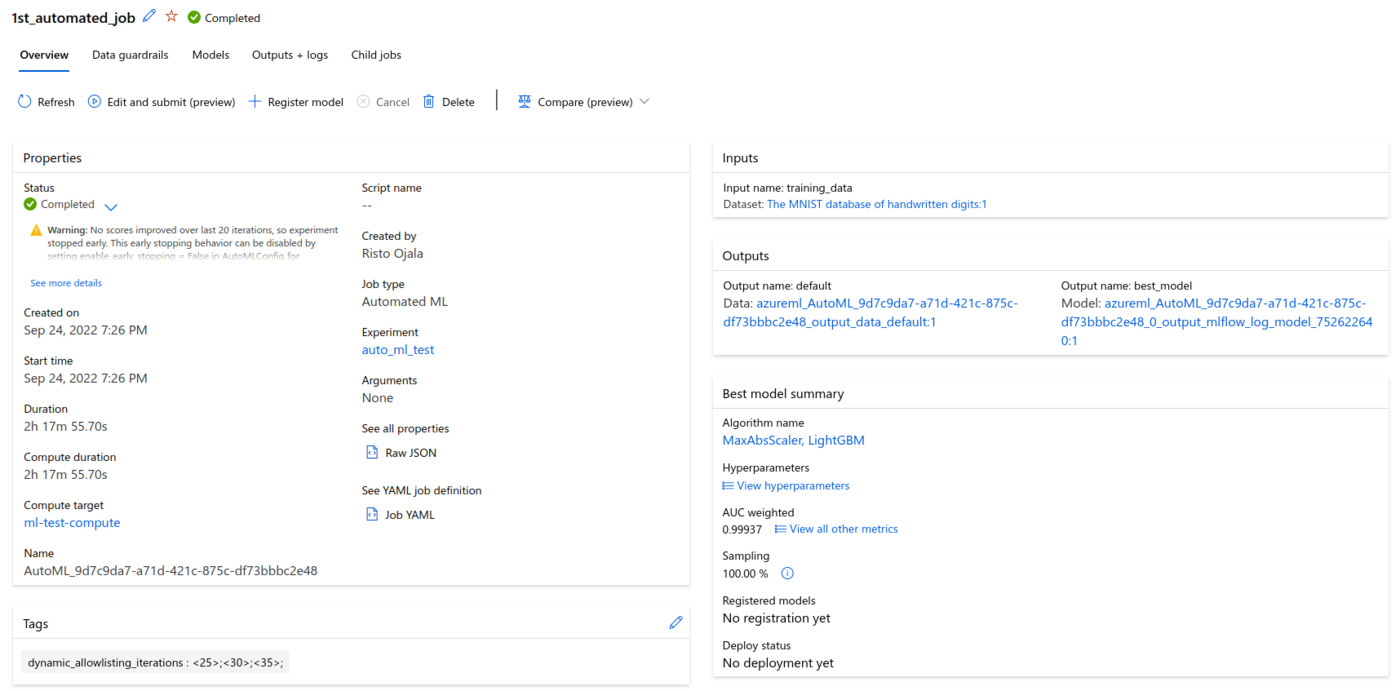
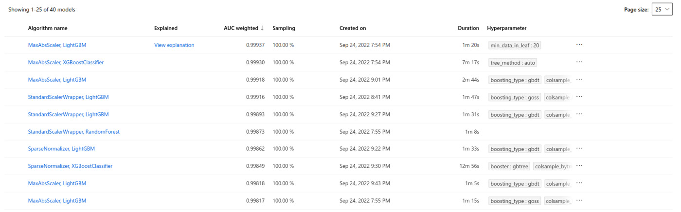
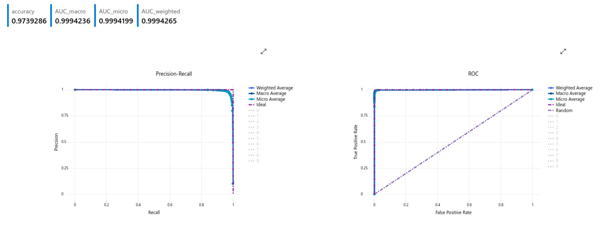
Contrary to my expectations, the job was finished in a bit over two hours. The system was clever enough to notice that the results weren’t improving, as the MNIST dataset is not much of the challenge for the classifiers. Over 0.99 weighted area under the ROC curve was reached consistently by the different classifiers and their different hyperparameter setups, basically showing flawless classification performance. A total of 40 different models were trained and validated, ranging from simple logistic regression to more advanced boosted classifiers. No deep learning models were trained yet, those are likely left as the last ones on the list of models to try, which is of course clever. The highest scoring algorithm was an implementation of gradient boosted decision trees (LightGBM) with simple MaxAbsScaler preprocessing.

Looking at the validation results for the algorithm, the nearly perfect classication result can be witnessed in the precision-recall and ROC curves (below).

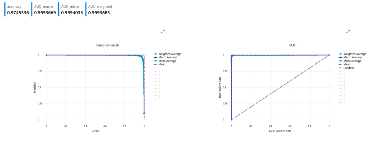
The test results were remarkably similar, further showing the capabilities of the algorithm.

So, pretty much the algorithm seemed more than suitable for the task, and the Automated ML job had performed its duty more than well. However, observing the calibration curve on the validation set, there was still some room for improvement. The predicted probabilities of the classifier were not entirely reliable. Although they clearly correlated with the proportion of positive samples, there is some notable spread in the results.

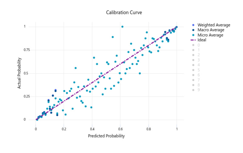
This is understandable considering that only the weighted AUC metric was utilised for ranking the models, so naturally the chosen model might not be perfect on all metrics. Still, I think it’s a good example that multiple metrics should always be considered when ranking different models. Especially if model selection is performed in an automated manner.

Final Notes

The job I performed was left a little short due to the classification task not being that challenging. On a more difficult task, the Automated ML system would have to iterate thousands of model, each with practically an infinite number of hyperparameter configurations. The explorable model/parameter space is so enormous, that it would be interesting to know what type of optimisation strategies the Automated ML module employs to find the possibly well-performing models. It is of course possible that a list of algorithms and hyperparameters is exhaustively iterated, yet that feels a bit brute-force. I’d assume that they have something more sophisticated for exploring the search space. They might also narrow the search by analysing the characteristics of the data, eg. the number of data samples and the number of features. This would allow to conveniently determine a ballpark for what type of models and hyperparameter configurations could handle the task.